
The accuracy for a point measured using an Intersection method is determined by three inter-related factors:
the separation of the Stations (Base Line),
the Angle of Intersection and
the Precision of the Angular Measurements.
Today high accuracy non-contact measurement can be achieved using Scanners and Reflectorless Total Stations where the accuracy of the measured points is determined by the precision of both the angular and distance measurements. However, these methods require considerable investment and Intersection methods such as Theodolite Intersection, Plane Table Surveying, Stereo Photogrammetry, Photographic Intersection and Spherical (360°) Panorama Intersection all provide low cost solutions. I have include methods using Theodolites as low cost because it is now possible to acquire these opto-mechanical instruments for similar prices to the cost of a DISTO.
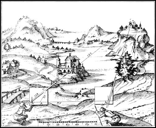 The illustration from “Novum Instrumentum Geometricum” by Leonhard Zubler of Zurich, published in 1614 by Ludwig Konigs of Basle, shows that the technique has been in existence for centuries.
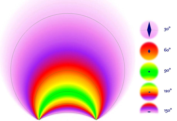
The highest accuracy when using Intersection is achieved when the measured point is on the sphere defined by the Stations being at either end of its diameter as here the rays intersect at a right angle and the error footprint is at its smallest.
The error footprint will increase as the Base Line increases, but the accuracy of a point on this sphere is also dependent on the precision of the Angular Measurements.
For example; for a point on the optimum sphere with a Base Line of 10 metres with Intersection using a 1″ Theodolite will give a theoretical error of around 0.1mm, whilst using 100MP Equirectangular images (pixel separation approximately 1.5 minutes of arc) will give a theoretical error of less than 10 mm. If the Base Line for the measurement using the 100MP Equirectangulars is reduced to one metre then we can expect an error of around 1mm.
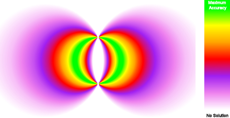
The error footprint increases in size as the measured point moves away from the optimum sphere, but as can be seen in the following image, there is considerable more increase in size as it moves away from the Base Line than towards it.
The following image shows the relative shape and size of the error footprint for Intersection Angles at 30° intervals:
 The following image provides an indication of the useful area for Intersection solutions:
 It is clear that whilst a short Base Line increases accuracy that the space where the accuracy can be achieved is much more restricted than for a longer Base Line as demonstrated by the following image:
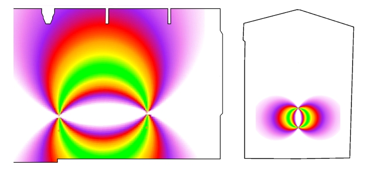 Given that the same tools are used in the above example for both the horizontally separated Stations shown on the left (plan) and the vertically separated Stations shown on the right (section) the accuracy of the points in the green zone for the horizontally separated Stations with the much longer Base Line will be somewhat poorer than the accuracy for the points in the green zone for the vertically separated Stations, but many more useful points can be measured to a reasonable degree of accuracy with the longer Base Line.
![]()