Introduction
The use of photography as a measurement tool has long been an interest of mine, and it is thirty eight years since I filed and was granted a patent for a device to photograph a complete horizon 360° panorama with a single exposure. The idea germinated a year earlier when I was looking for a photographic method to measure a myriad of rooms at Annesley Hall in Nottinghamshire, England, and developed from a property of using a fisheye lens looking vertically so that the image is in a horizontal plane. This property is that all the directions from the centre of the image were true so that an angle subtended by two points in the image at the centre was the same as on the ground. The advantage of using photography for measurement is that all the information in the photograph is available for future use without having to revisit the site, which may no longer exist.
 The use of the image from the fisheye lens had a major drawback in that most of the information of interest is restricted to a narrow band round the circumference. Although both computers and digital imaging existed in the mid 1970s, they were prohibitively expensive so not in the public domain and the personal computer and affordable digital camera were science fiction, so the only way to utilise this process was to make a print to use as a protractor. These technologies are ready available today and talented people have created the software and hardware that enable us to enjoy the creation of Spherical (360°) Panoramas.
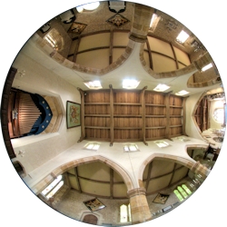
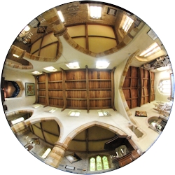
Spherical Panorama images are actually projections so have different geometrical properties to photographs, and projections such as the “Little Planet” and “Mirror Ball” from Pano2VR and “Polar”, “Mirror Ball” and “Magnipolar” from flaming pear have the same property as the fisheye lens looking vertically and that of my “Optic for Instantaneously Photographing an Horizon of 360°” in that when they are created looking vertically down (i.e. to the nadir, -90°) all the directions from the centre are true.
![]()
Basic Principles
The basic principle of Photogrammetry, of which Photographic Intersection is a special case, is that if we have two or more directions in space that have know origins we can calculate the position of that point. The accuracy with which we can do this is very dependent of the angles those rays intersect at. Maximum accuracy is achieved when the angle of intersection is a right angle and deteriorates as the angle become more acute or obtuse, until there is no solution as described further on.
The position of the points from which the directions begin are determined by conventional surveying (geomatics) techniques and can be measured directly or by resecting their positions from Control Points with known positions, or both. Techniques used before the advent of EDM (Electromagnetic Distance Measurements) can be employed as Photogrammetry is essentially an angle measurement process, but at least one distance measurement must be included for scale. This could be the distance between two camera locations or two Control Points and should be of reasonable length in relation to the area being measured.
To use photographs for measurement we need to take into account such parameters as focal length of the lens, sensor dimensions (whether film or digital) and lens distortions including the location of the entrance pupil which can change with the angle the light enters the lens. With metric cameras, such as the Wild P31 and Wild P32 lens distortion is virtually non-existent (just a few microns in the corner of a large format) and they have a single entrance pupil, so they are much easier to deal with, but were hugely expensive and no longer available.
Spherical Panorama images are projections so are much simpler to deal with than photographs as they always have a single point of origin and a structured geometry. We can think of a Spherical Panorama in the same way as the Celestial Sphere. We know that the stars are not on a sphere with the earth at the centre, but we can treat them as such for navigation and position determination. We can reference each star by its Declination (angle above and below the ecliptic) and its Right Ascension (angle along the ecliptic from the reference point know as the First Point of Aries) at a given point in time. This data can be extracted from a Star Almanac. The ecliptic is the imaginary plane in which the planets of our solar system revolve around our sun. The predictability of the position of the stars on the Celestial Sphere can be used to calibrate lenses as described on John Houghton’s site. We can consider a Spherical Panorama in in the same way with the horizontal plane through the panorama equivalent to the ecliptic, the angles above and below this horizon as Vertical Angles and the angles around this horizon as Horizontal Angles referenced to a known point in exactly the same way as if we used a theodolite.
![]()
Using the Equirectangular Projection for Measurement
 The Equirectangular Projection is usually the first step in creating the Spherical Panorama from the recorded images with software such as PTGui or Immersive Studio, so is readily available. This projection is attributed to Marinus of Tyre in 100AD and has the property that meridians are equally spaced vertical lines and the circles of latitude are equally spaced horizontal lines making it ideal for measuring directions from the projection centre, but not very suitable for mapping for either navigation or cadastre because of the distortions.
A property of the Equirectangular Projection is that the pixel separation can be directly interpreted as an angle and that the values are the same both vertically and horizontally. If we have a very low resolution Equirectangular image of 360 x 180 pixels then the separation between each pixel both vertically and horizontally is one degree of arc. An image of 3,600 x 1,800, which is easily attainable, will have an angle separation of 0.1 degrees = 6 minutes of arc, which equates to 17mm at 10m. This means that the pixel co-ordinates of a point in the image can be translated into a Vertical Angle relative to the central horizontal axis of the projection and a Horizontal Angle relative to a reference point in the image by simple arithmetic. Calculations can easily be made using a simple calculator or a spread sheet, such as Excel. An Equirectangular image can be looked upon as a photographic theodolite.
Once the angles have been derived they can be used to graphically plot the points of interest or used to compute their co-ordinates relative to the known points using the same mathematics as for theodolite intersection. The angles can be plotted as with Plane Table surveying or using a software package such as LISCAD.
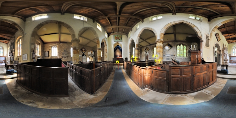
The following example uses two 10,000 x 5,000 Equirectangular images taken 5.98m apart with a reference target at each of the two locations. The 10,000 x 5,000 Equirectangular gives a pixel separation both horizontally and vertically of just over two minutes of arc and equates to some 6mm at 10m.
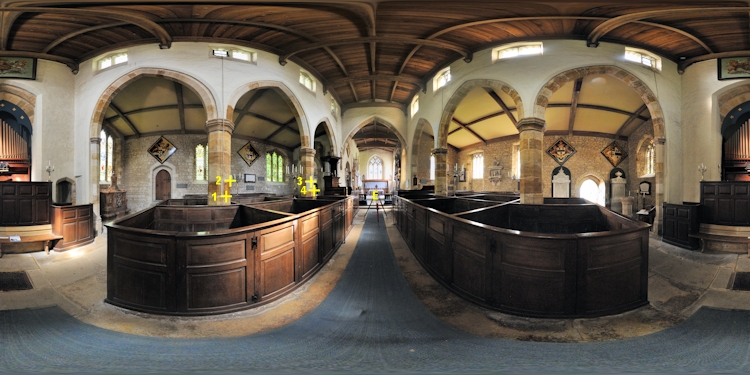
The angles are derived as follows:
Horizontal Angle = (horizontal pixel difference between the reference and the point / horizontal pixels for the image) x 360
Vertical Angle = (vertical pixel difference between the horizon and the point / vertical pixels for the image) x 180
e.g.
Horizontal Angle for point 1 from W = ( ( 2890 – 5018 ) / 10000 ) x 360
Vertical Angle for point 1 from W = ( ( 2622 – 2500 ) / 5000) x 180
| Point | Horizontal | Vertical | Horizontal | Vertical | Horizontal | Vertical |
| Pixel | Pixel | Difference | Difference | Angle ° | Angle ° | |
| Data from W | ||||||
| E | 5018 | 2487 | 0 | -13 | 0.000 | -0.468 |
| 1 | 2890 | 2622 | -2128 | 122 | -76.608 | 4.392 |
| 2 | 3012 | 2419 | -2006 | -81 | -72.216 | -2.916 |
| 3 | 4144 | 2421 | -874 | -79 | -31.464 | -2.844 |
| 4 | 4180 | 2540 | -838 | 40 | -30.168 | 1.440 |
| Data from E | ||||||
| W | 5001 | 2497 | 0 | -3 | 0.000 | -0.108 |
| 1 | 5727 | 2545 | 726 | 45 | 26.136 | 1.620 |
| 2 | 5751 | 2450 | 750 | -50 | 27.000 | -1.800 |
| 3 | 6649 | 2378 | 1648 | -122 | 59.328 | -4.392 |
| 4 | 6745 | 2575 | 1744 | 75 | 62.784 | 2.700 |
![]()
Using the Other Projections for Measurement
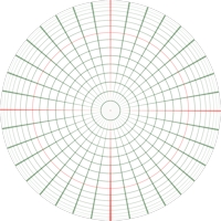
Once the Equirectangular Projection has been created it can be transformed into a huge variety of projections, some of which have the property that the directions from the centre are exactly the same in the projection as from the same location on site so that Horizontal Angles can be readily determined. These include “Little Planet” and “Mirror Ball” from Pano2VR and “Polar”, “Mirror Ball” and “Magnipolar” from flaming pear. The “Little Planet” projection from Pano2VR and the “Polar” projection from flaming pear, as shown in the diagram to the right, also have the property that the Vertical Angle is proportional to the radius for a particular point. With the “Little Planet” and “Polar” projections the meridians radiate from the centre as straight lines with their correct angular separation and the circles of latitude are equally spaced circles making it ideal for measurement, but again impractical for mapping. As with the Equirectangular Projection, the pixel co-ordinates of a point in these image can be easily translated into a Vertical Angle relative to the centre of the projection and a Horizontal Angle relative to a reference point in the image, by simple arithmetic and a little trigonometry.
As with the data from the Equirectangular Projection, once the angles have been derived they can be used to graphically plot the points of interest or used to compute their co-ordinates relative to the known points. However, these projections can also be used as “protractors” to plot the intersection rays from the locations of the Spherical Panoramas. Mapping packages, such as LISCAD have the ability to import images as a background and use them to build up the map.
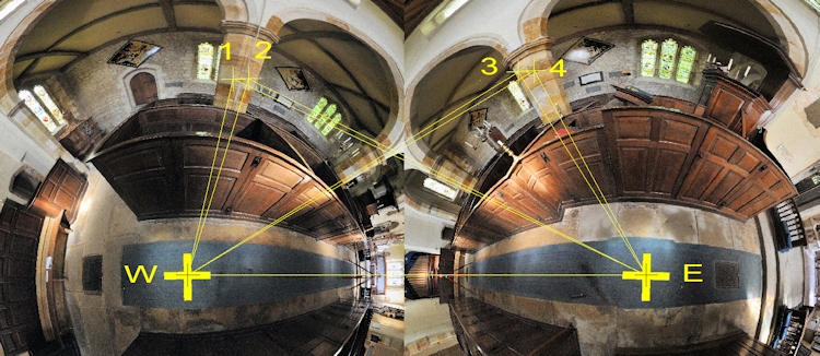
In the following example the two “Stations” were created in LISCAD separated by the 5.98m measured between them on site and the two “Little Planet” projections imported using the “Background Images” option and fitted to the two “Stations” and orientated to the targeted reference points. The directions were then used to compute the detail points by intersection.
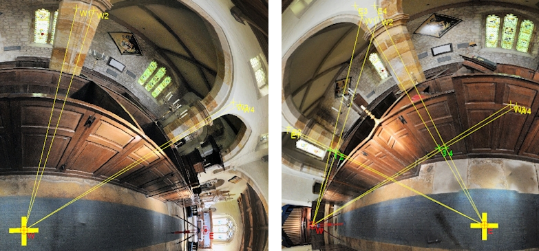
First, one Little Planet projection is fitted to one Station and the rays drawn from the centre through the points of interest. Note that the rays pass some way through the points of interest to give maximum accuracy. The second Little Planet projection is then fitted to the other Station and the rays again drawn through the points of interest from the centre. The points of interest are then computed by the intersection of these rays. The higher the resolution of the Little Planet Projections used, the better will be the accuracy.
The following image has been included to illustrate the process using lower resolution Little Planet projections.
 The data values could also have be computed from the pixel co-ordinates in much the same way as for the Equirectangular projection method, the difference being that the Horizontal Angles will be derived using trigonometry as:
tan (Horizontal Angle|) = (horizontal pixel difference / vertical pixel difference)
and the Vertical Angle derived by Pythagoras as it is the radial difference from the circle representing the horizontal plane through the projection divided by the radius of the projection multiplied by 180°. This calculation for the Vertical Angle only applies to the Little Planet projection (Pano2VR) and the Polar projection (flaming pear). The other projections will require more complex calculations for determining the Vertical Angles because the the lines of latitude are not equally spaced in these projections, as shown by the Mirror Ball projection to the right.
The mathematics for determining the Horizontal and Vertical angles to the points of interest with the Equirectangular projection is much more straight forward than with these other protections so I would suggest it is the preferred option, but these other projections may be preferred if using a graphical solution or using software, such as LISCAD, to provide the results. The angle of cut (intersection) is more readily recognised using these other projections than with the Equirectangular projection, which is pertinent to the accuracy of the measured point as mentioned following.![]()
Vertically Separated Spherical Panoramas
The example above uses two horizontally separated panoramas, but the panoramas can be separated vertically, as used in the Spheron solution.
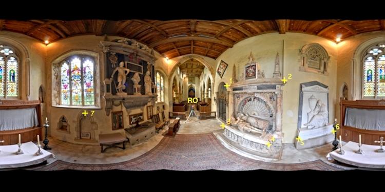
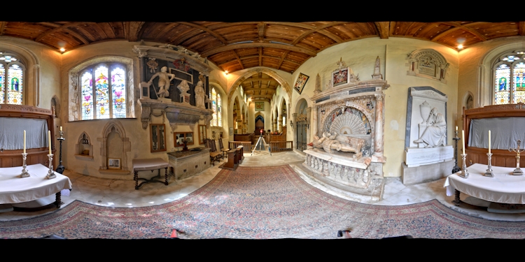
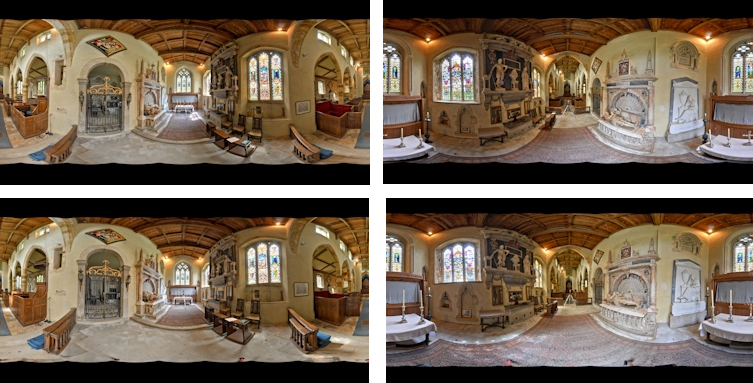
The two following images show the “high” and “low” panoramas taken using a tripod supported pole for rigidity. Note that no attempt has been made to include the zenith and nadir for these panoramas because these areas are in the “no solution” zones for intersection.
The following example uses two 10,000 x 5,000 Equirectangular images taken 1.00m apart vertically, with a common reference target. The 10,000 x 5,000 Equirectangular gives a pixel separation both horizontally and vertically of just over two minutes of arc and equates to some 6mm at 10m.
The Horizontal and Vertical Angle data is extracted in exactly the same way as for the horizontally separated panoramas.
The angles are derived as follows:
Horizontal Angle = (horizontal pixel difference between the reference and the point / horizontal pixels for the image) x 360
Vertical Angle = (vertical pixel difference between the horizon and the point / vertical pixels for the image) x 180
e.g.
Horizontal Angle for point 1 from High = ( ( 5903 – 5010 ) / 10000 ) x 360
Vertical Angle for point 1 from Low = ( ( 2243 – 2500 ) / 5000) x 180
| Point | Horizontal | Vertical | Horizontal | Vertical | Horizontal | Vertical |
| Pixel | Pixel | Difference | Difference | Angle ° | Angle ° | |
| Data from | High | |||||
| RO | 5010 | 2769 | 0 | 269 | 0.000 | 9.684 |
| 1 | 5903 | 2243 | 893 | -257 | 32.148 | -9.252 |
| 2 | 7392 | 2094 | 2382 | -406 | 85.752 | -14.616 |
| 3 | 5797 | 3284 | 787 | 784 | 28.332 | 28.224 |
| 4 | 6980 | 3773 | 1970 | 1273 | 70.920 | 45.828 |
| 5 | 7757 | 3624 | 2747 | 1124 | 98.892 | 40.464 |
| 6 | 8667 | 3415 | 3657 | 915 | 131.652 | 32.940 |
| 7 | 2197 | 2950 | -2813 | 450 | -101.268 | 16.200 |
| Data from | Low | |||||
| RO | 4978 | 2505 | 0 | 5 | 0.000 | 0.180 |
| 1 | 5875 | 1881 | 897 | -619 | 32.292 | -22.284 |
| 2 | 7376 | 1532 | 2398 | -968 | 86.328 | -34.848 |
| 3 | 5768 | 2890 | 790 | 390 | 28.440 | 14.040 |
| 4 | 6965 | 3227 | 1987 | 727 | 71.532 | 26.172 |
| 5 | 7741 | 3141 | 2763 | 641 | 99.468 | 23.076 |
| 6 | 8642 | 3002 | 3664 | 502 | 131.904 | 18.072 |
| 7 | 2153 | 2399 | -2825 | -101 | -101.700 | -3.636 |
Advantages of using vertically separated spherical panoramas are that the targeted reference point is common and the similarity between the two panoramas makes for much easier identification of the points of interest from each.
The disadvantage is that the base is usually much shorter because of the equipment required to lift the camera from the Low position to the High position. In this example the base is just 1m compared with 6m for the horizontally placed panoramas. This clearly will influence the accuracy because the region of maximum accuracy will be much closer to the panoramas.
Accuracy and coverage can be improved by combining both horizontally and vertically separated panoramas.
In theory, if an arrangement as shown above is used, where the “other” location is targeted, the only distance measurements required are the two vertical bases as the distances between the horizontal locations can be calculated from the Vertical Angle information for each vertically separated pair. However, for a 6m horizontal base with a 1m vertical base the the angle of intersection is just less than 10° at best (i.e. if the target is at the same height as the mid point between the two vertically separated panoramas), so accuracy will be severely compromised. To give an idea of how much, a 2mm error in the vertical base coupled with an angular error subtended by two pixels can result in a 0.15m error in the horizontal base distance. It is important to have good measurements to scale the model and suitable values are the distance between the two horizontal panoramas or two or more Control Points separated by a similar amount or preferably both as this will provide a check on the precision of the data extraction.
A practical solution is to use the arrangement shown above, but computing all four horizontal arrangements. i.e. High Left with High Right, High Left with Low Right, Low Left with High Right and Low Left with Low Right. The mean from the four solutions will give a stronger result and the “spread” from the four results will give a good idea of the precision of the measurements.
The panoramas used in this example have a resolution of 10000 x 5000 pixels and a horizontal base of 6m. To give some idea of the precision of this form of measurement the results showed that the average distance from the mean value to the individual measured points was some 6mm maximising at 10mm where there were good angles of intersection. This value rose to 20mm in the “orange/red” regions where the angle of intersection fell below 70°.![]()
Accuracy
Accuracy is clearly a function of the resolution of the images being used, as illustrated in the text relating to using the Equirectangular Projection, as the higher the resolution the smaller the angle separation between adjacent pixels. Accuracy is also dependent on the nature of the points being measured. “Hard” detail points are easier to select than “softer” points and easier to identify in different panoramas. However, as previously mentioned, it is also directly related to the angel of intersection of the rays in space. Maximum accuracy is achieved when the angle of intersection is a right angle and deteriorates as the angle become more acute or obtuse, until there is no solution.
The diagram below shows how important it is to consider the locations for the Spherical Panoramas to achieve the best results. Note that this applies to both horizontally and vertically displaced panoramas. This criteria is the same for Stereo Photogrammetry and Photographic Intersection, but in these applications the field of view of the lens controls the area captured in the image. The difference with using the projections from Spherical Panoramas is that we capture a full 360° horizon so can measure points both sides of the axis between the panoramas.
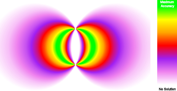
Placing the accuracy diagram in relation to the two Spherical Panorama locations, used in the first example, in the building demonstrates the importance of ensuring that the Spherical Panoramas are taken in the right places.
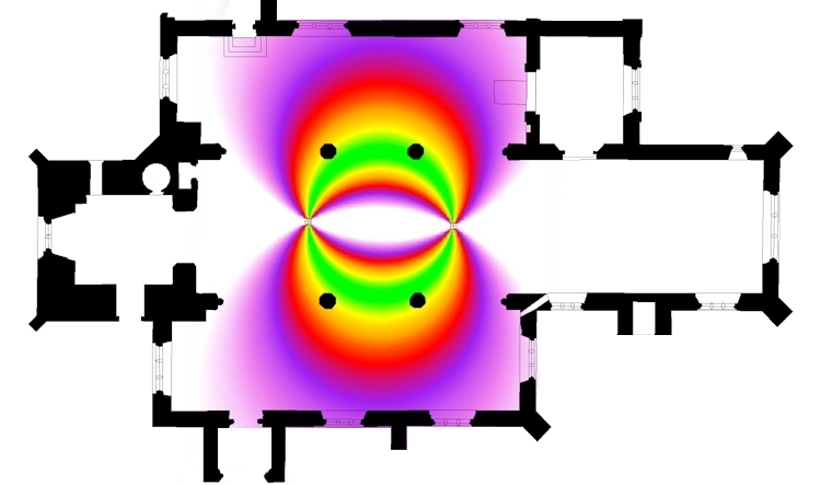
The following diagrams shows the difference in accuracy coverage in plan and elevation between the two horizontal panorama locations with a 6m base compared with that for the two vertically separated panoramas with a one metre base.
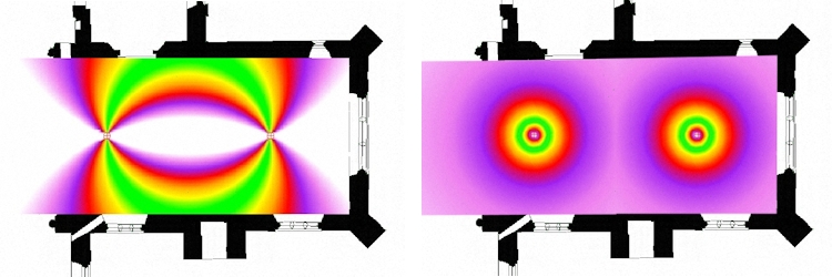
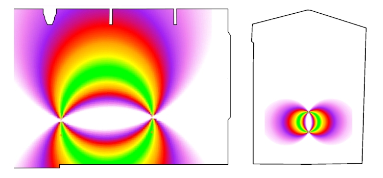
…and yes, the wall on the right in the right hand diagram does lean like that! The weight of the enormous monument on the south wall is supported by a substantial external buttress.
![]()